Continental Hotspot

In this post we’ll be delving into the leading theory of modified gravity called Modified Newtonian Dynamics, MOND for short. This theory was first developed by Mordehai Milgrom in a series of papers in 1983. In its simplest form MOND is an algorithm to determine the observed gravitational accelerations from the observed distribution of matter in the universe and vice versa. MOND is simpler and much more restrictive than dark matter because dark matter which is invisible could in principle have any distribution. Yet MOND can fit and predict a great many observations.

First we’ll talk some history, then we’ll look into what sort of environment MOND applies in, what the “interpolation function” is and what the MOND field equations are. To cap it off we look at a simple example of a galaxy rotation curve.

Before we dive in a note on the terminology. MOND which is an acronym for Modified Newtonian Dynamics is more and more often being referred to as Milgromian dynamics instead, after Mordehai Milgrom who came up with the theory. There are two reasons for this. The most important is that in recent years many relativistic versions of this theory have been proposed so it is no longer quite accurate to call it a modification of Newtonian dynamics. Another reason that some researchers have pointed out is that Modified Newtonian Dynamics implies that the dynamics themselves are being modified and not our description of them which is weird since the laws of nature don’t care how well we understand them. In this guide I’ll be using both MOND and Milgromian dynamics interchangeably. Personally I prefer Milgromian dynamics but it is somewhat longer and the acronym is also still more widely known.

History

Starting in the early 20th century astronomers started noticing that certain objects in the universe were not behaving as they should. Oort noticed that stars in the Milky Way were moving too fast. Zwicky noticed that galaxies in galaxy clusters were moving way too fast. And starting in the 1970s first Vera Rubin in optical data and then Albert Bosma in radio measurements noticed that rotation curves of galaxies other than our own Milky Way were becoming flat out towards the edges of those galaxies. These and several more puzzling phenomena that were discovered later were discussed in the first post of this series.

With all of these discrepancies between the observed mass and the observed movements piling up, in 1981 along comes Professor Mordehai “Moti” Milgrom then at the Institute for Advanced Study in Princeton now at the Weizmann Institute of Science. Over the course of two years he compared a range of different possible modifications of the laws of gravity as we know them to check if such modifications could replicate the observed flatness of rotation curves. He settled on a modification based on an acceleration scale which he then published in three foundational papers which outlined his new theory:

• A modification of the Newtonian dynamics as a possible alternative to the hidden mass hypothesis
• A modification of the Newtonian dynamics: Implications for galaxies
• A modification of the newtonian dynamics: Implications for galaxy systems

A further fundamental paper was published a year later in 1984 when Mordehai Milgrom was joined by world renowned physicist and his good friend Jacob Bekenstein in which they propose the first field equations as derived from a Lagrangian. Having such a foundation for the theory was very important because it ensured that energy and momentum conservation would be satisfied. Another post will go into all this on a later date so I won’t elaborate on it here.

• Does the missing mass problem signal the breakdown of Newtonian gravity?

From the 1990s onward a number of very influential astronomers, astrophysicists and cosmologists have joined Milgrom in his pursuit of this research. At some point I’ll do a post on who’s who to cover more people and their work than I can mention here. For now I’ll only drop the names of Bob Sanders and Stacy McGaugh who risked their careers to join the work on what was then a fringe theory.

Since then the research on Milgromian dynamics has bloomed into an active and growing field of research. A number of large conferences have been held on the topic. The most recent one at the time of this writing was the MOND40 conference in St. Andrews, Scotland, held in June of 2023.

Regime where MOND applies

Ok so MOND is a new theory of gravity posited by Mordehai Milgrom which has attracted quite a number of people to it over the years. But when does it apply and what does it actually say should happen?

MOND is something like a patch for Newtonian gravity that already works well on Earth and in the Solar system. Given the appropriate circumstances MOND encapsulates Newtonian gravity. In this sense it is similar to general relativity (GR) which also contains Newtonian gravity as a limit. MOND applies when velocities are much slower than the speed of light and the gravitational potential is small. GR on the other hand applies when gravitational accelerations are larger than Milgrom’s constant a₀ (or if you believe in dark matter, GR applies everywhere). Mathematically this can be summarized by the following limits:

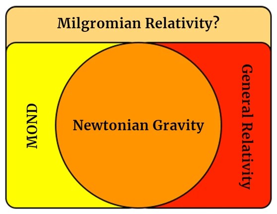
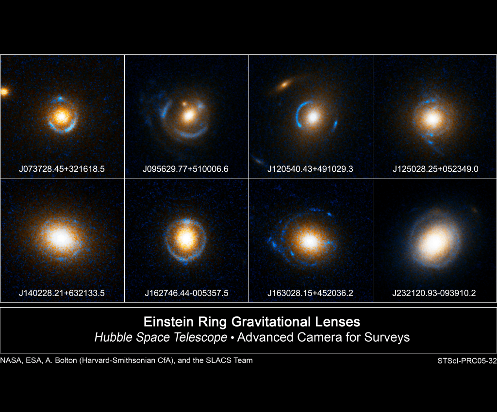
MOND is not a relativistic theory and cannot explain relativistic phenomena like gravitational lensing or the expansion of the universe. For that an additional theory would be required which unifies MOND with GR in a sort of “Milgromian Relativity” (many attempts at this have been proposed though none has been truly convincing so far).

That may still seem abstract. In what sort of systems do we really see MOND differ from GR or from high school Newtonian gravity? The most prominent example is in galaxies as we’ve discussed in the first post of this series. To give a bit of perspective look how different the environment is in a galaxy compared to every day life:

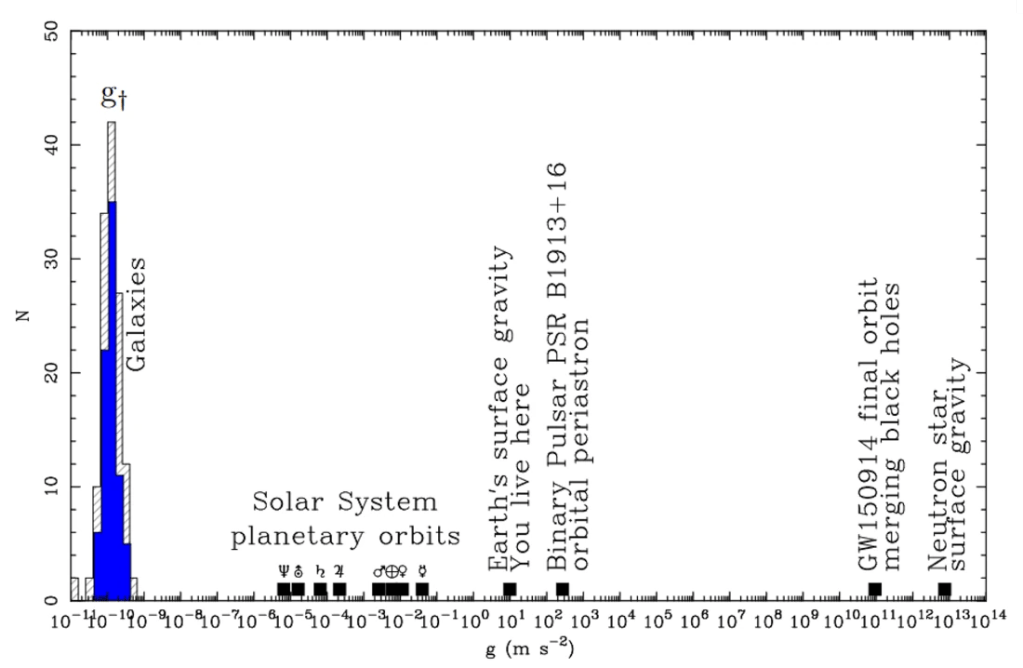
MOND shows differences when the gravity is a trillion times weaker than here on Earth!

The interpolating function

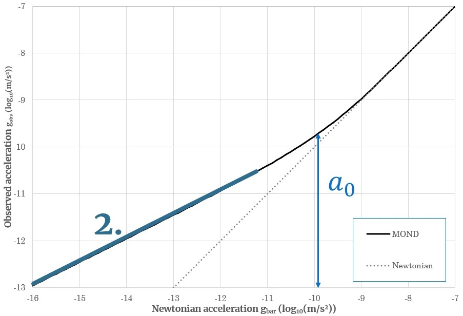
To really get to grips with MOND we need to dissect the diagram below. We’ll do this in steps just like the animation shows and work our way up to what is known as the “interpolation function”. This interpolation function is the algorithm which allows MOND to calculate the movement of mass from its distribution and the other way around.

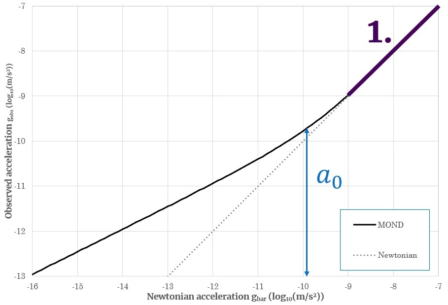
Along the horizontal axis we have the ordinary Newtonian gravitational acceleration determined by how much mass we observe there to be and then applying Newton’s Law of Universal Gravitation. Along the vertical axis we have the observed gravitational acceleration. This can be determined from how fast things are moving at a given radius and how strongly light is bent around an object. This plot is logarithmic though so for each grid cell you move towards the lower left corner the weaker the accelerations gets by a factor of 10. The typical gravitational accelerations in the solar system (of the sun on the planets or the Earth on us) are way too big to fit on this plot and those would be way off to the top right of your screen.

Next let’s look at the first three lines. The dotted line is the line where we expect all the data to fall on if Newtonian gravity (and GR) were correct and dark matter doesn’t exist (also indicated with a thick red line in the animation). The full black line with the bend in it around 10^-10 m/s² is the expectation from MOND. The dashed line shows the limit of how gravity behaves according to MOND if it gets super weak. This line is merely there to illustrate that the MOND curve approaches a straight line in this log-log plot at gravitational accelerations below ~10^-10 m/s².

Now let’s look at the acceleration denoted by the red arrow and “a₀“. MOND says that this is a threshold acceleration defined by Milgrom’s constant a₀ at 1.2 x 10^-10 m/s². Below this acceleration the gravity is stronger than expected and gets a boost in strength compared to what Newton would predict (indicated by the red arrow starting at the dotted Newtonian line). Above this acceleration gravity behaves as Newton would predict.

This MOND expectation is an excellent fit for the data and in many cases preceded the data begin gathered by several decades. The plot shows several different data types. The dark blue diamonds show large elliptical galaxies which are supported by random and chaotic motions of stars. The light blue squares overlapping them are binned results for spiral disk galaxies that rotate in a very structured way as measured in a rotation curve. Both of these data sets can be found in this paper by Lelli et al. Down towards the low end the data with error bars comes from a recent study by Brouwer et al. using weak gravitational lensing in the furthest reaches around very isolated galaxies. Even though MOND is not a relativistic theory and hence cannot account for gravitational lensing through spacetime curvature, when the data is expressed in terms of the relevant strength of gravity we see that the data nonetheless follows the Milgromian expectation.

The black curve in the animation above has several names but the most important two are the “Radial Acceleration Relation (RAR)” and “Milgrom’s law”. The former is a neutral phenomenological name for the trend in the data. The latter is the name for the behaviour predicted by Milgrom in the first foundational paper in 1983.

The fact that the data so closely follows Milgrom’s prediction from 1983 is rather remarkable from the perspective of dark matter. Because dark matter could in principle have any distribution compared to the distribution of ordinary matter (often called baryonic matter because most stuff you know is made up of baryons) because there are many effects such as ordinary matter collisions, supernova and AGN feedback, and the efficiency of that feedback, dark matter self-interaction, Chandrasekhar friction and so on that could change the distribution of dark matter compared to normal matter. All that means that with ordinary GR and dark matter observations could lie anywhere above the dotted line (in the blue shaded area). But it doesn’t. The data neatly falls right on Milgrom’s law.

The two most important limits of Milgrom’s law are the Newtonian limit (denoted by the purple 1 in the graphs below) and the Milgromian, or Deep-MOND, limit (denoted by the blue 2). In between is a transition region right around a₀ where the two curves smoothly flow into each other.

This smooth transition and hence Milgrom’s law is defined using the interpolation function of MOND. Several have been proposed in the literature, all with the same limits and slightly different behaviour around a₀. In this series I’ll stick to what is known as the “simple” interpolation function. In general we can express this interpolation function in two mathematically equivalent directions. On the one hand to calculate the observed mass distribution from the dynamics and on the other to calculate the movement of mass and light to the distribution of matter.

Below follow the proofs that the Newtonian and Milgromian limits hold for the simple interpolation function. In these equations g_M stands for the dynamical acceleration as measured from the movement or bending of light. It is also often called g_obs. The acceleration from the distribution of mass is denoted by g_N but is also often called g_bar.

1. The Newtonian limit

In this limit of MOND gravity behaves just like it does in the solar system. It happens when gravity is (much) stronger than Milgrom’s constant a₀.

2. The Milgromian limit (Deep-MOND limit)

In this limit of MOND gravity is stronger than would be expected in Newtonian gravity. This occurs almost exclusively in astronomical systems because only then the gravitational fields become low enough.

Field equations

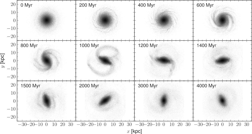
The equations above are really only for a one-dimensional case and well.. the universe isn’t one dimensional. In many symmetrical cases those equations work just fine but suppose we have more complicated systems that are not symmetrical and/or are changing over time we really need so-called field equations. These describe the universe fully and can be used to simulate complex systems such as the spiral arms in the graph below.

In MOND the field equation is a modified version of Poisson’s equation. There are actually two ways to approach in the same fashion as using either μ or 𝜈. The QUMOND field equation can be solved numerically with codes like Phantom of Ramses. The AQUAL field equation is less complex algebraically but has to be solved iteratively because |∇ϕ| appears twice. AQUAL and QUMOND do give slightly different predictions on the order of 1-10% depending on the problem being analysed. For most applications both are equivalent however.

The derivation of these field equations from the Lagrangian will be covered in another post. Similarly the possible relativistic theories that reduce to these field equations in the appropriate limits will be discussed later.

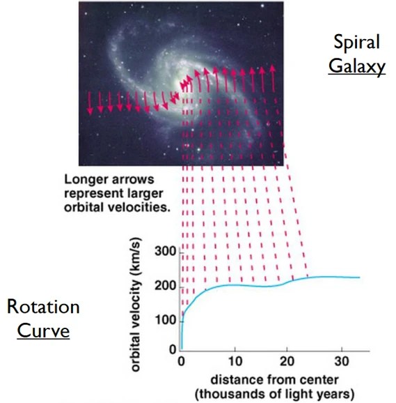
An example: MOND in a galaxy

In a disk galaxy the dynamical acceleration can be determined by first measuring the rotational velocities of the disk in a rotation curve as shown in the image below. Then the dynamical acceleration equal the velocity squared divided by the radius: g_M=g_obs=V²/R. The baryonic acceleration from the mass distribution can be calculated by the mass from the stars and gas, multiplying by Newton’s constant and dividing by the square of the radius: g_N=g_bar=GM/R². This simplifies matters a bit because that technically only holds for a sphere and disks rotate slightly faster but it is a pretty good first approximation. To get such measurements one also has to take into account various factors such as the inclination of the disk to the observer, the distance and the mass-to-light ratio of the stars all of which can be constrained by further measurements and reference models.

Once you either have g_M or g_N you can use MOND to predict the other. MOND has been able to do this for many galaxies, in advance of the actual measurement thus achieving the gold standard of scientific prediction. Alternatively you can measure both and plot the data on a log-log plot to see if it falls on Milgrom’s law.